Comparison of NonLinLoc and linear earthquake locations in a 3D model.
Anthony Lomax
Geosciences-Azur, 250 rue Albert Einstein, 06560 Valbonne, France; anthony@alomax.net, http://www.alomax.net/science
Alberto Michelini
Istituto Nazionale di Oceanografia e di Geofisica Sperimentale, Borgo Grotta Gigante 42/c, 34010 Sgonico, Trieste, Italy; michelini@ogs.trieste.it
May 2001
Abstract
We compare the global-search earthquake location method NonLinLoc (Lomax et al., 2000; http://www.alomax.net/nlloc) with the standard, iterative-linear method adopted by Thurber (1983) and Michelini and McEvilly (1991) using aftershock locations for the M=7, 1989 Loma-Prieta, California earthquake. For both methods we use the same 3D model and L2 misfit function. The differences in hypocentral co-ordinates between the two methods are typically of the same order or smaller than the spatial location uncertainty. Thus we can associate differences in the locations to differences in the model parameterisation, travel-time calculation and optimisation algorithms of the two methods, and we conclude that the two sets of locations are compatible.
Introduction
Earthquake location in 3D models can be performed with iterative-linear inversion or with non-linear global search methods. Typically, estimates of the location uncertainty will be different for the two approaches. However, for well constrained events, when the same data-error model and misfit norm norm are used, and in the absence of strong velocity gradients in the model, the optimal or maximum likelihood hypocenters from the two approaches should be nearly identical.
In order to verify the performance of the the global-search, NonLinLoc location software (Lomax et al., 2000; http://www.alomax.net/nlloc), we compare optimal aftershock locations for the M=7, 1989 Loma-Prieta, California earthquake obtained using NonLinLoc and the standard, iterative-linear method of Michelini and McEvilly (1991) (M&McE91 hereafter). This latter method is the adaptation to cubic B-splines of the SIMULPS joint hypocenter/velocity structure inversion algorithms of Thurber (1983). For both methods we use (1) the same 3D, P velocity model for the Loma Prieta region (Michelini, 1991; Foxall et al., 1993), (2) the same L2 (least-squares) misfit function, and (3) identical, observed, P travel times from the Northern California Seismic Network for events of M>3 from 17Oct1989 to 17Oct1990, obtained from the Northern California Earthquake Data Center (http://quake.geo.berkeley.edu).
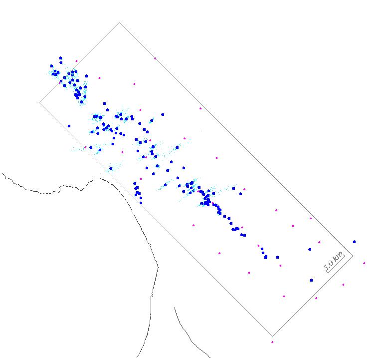
The locations are performed for all stations and events that fall within a model volume of 30km x 78km x 24km deep (Figure 1). For the M&McE91 method, the model is parameterized by cubic B-splines on a 9x11x6 grid with node spacing of 3km, 7km and 3km in the x, y and depth directions, respectively. For NonLinLoc, the model is parameterized by constant velocity, cubic cells of side 0.25km.
Figure 1. (blue dots) maximum likelihood point and (light blue clouds) probability density functions for all NonLinLoc hypocenters. (small violet dots) stations. Grey lines indicate limits of the 3D velocity model. Blakc lines show coastline and a fault structure.
Results
We consider the maximum-likelihood hypocenters (Figure 1) and associated Gaussian, 68%-confidence ellipsoids (Figure 2) obtained with NonLinLoc, and the optimal, least-squares hypocenters obtained with the linear M&McE91 inversion. We examine the results for 119 well-located events with at least 10 observations.

Figure 2. (red ellipsoids) 68% confidence ellipsoids for all NonLinLoc hypocenters. Grey lines indicate limits of the 3D velocity model. Lower view is a depth section from the Northeast.
The differences in hypocentral co-ordinates between the two methods (Figure 3) are typically of the same order or smaller than the spatial location uncertainty as indicated by the NonLinLoc confidence ellipsoids (Figure 2), except for some events with very small confidence ellipsoids. Confidence ellipsoids show the volume within which the location misfit function varies little from its minimum value. Thus a difference in hypocenter co-ordinates that is of the order of the size of the corresponding ellipsoid can be attributed to fundamental differences in the location algorithms and does not indicate an incompatibility in the results. In particular, the optimal hypocenters obtained with the two methods can be expected to differ because:
NonLinLoc uses a gridded representation of the 3D model consisting of constant velocity, cubic cells, while the M&McE91 method uses a smooth, cubic B-spline parameterisation.
To obtain calculated travel-times, NonLinLoc uses a grid-based, Huygens-principle, finite-difference algorithm (Podvin and Lecomte, 1991), while the M&McE91 algorithm uses the two-point, "ray bending" method proposed by Um and Thurber (1987) to find a minimum time ray.
NonLinLoc uses a stochastic, non-linear, directed, global-search to obtain the optimal (maximum-likelihood) hypocenter, while the M&McE91 method uses an iterative, least-squares minimisation of the linearized problem.

Figure 3. (blue line segments) difference between NonLinLoc and M&McE91 hypocenters for 119 well-located events with at least 10 observations. Grey lines indicate limits of the 3D velocity model. Lower view is a depth section from the Northeast.
Some events which have very small confidence ellipsoids show hypocentral differences between the two methods that are small, but larger than the ellipsoid size. This is most apparent for the events forming a linear trend at the Southeast of the study volume, and for events at intermediate depth in the middle of the study volume (compare Figures 2 and 3). In general, the differences in hypocenters for these events are locally of similar magnitude and orientation, but vary between different regions of the study volume. Thus these hypocentral differences may be attributed to the model parameterisation and consequent spatially varying travel time differences between the methods. This hypothesis is supported by the results of relocation with NonLinLoc of the events using a larger cell size for the model parameterization (0.5km vs. 0.25km) which produces larger hypocentral differences relative to the M&McE91 results.
Conclusions
We associate differences in the locations to differences in the model parameterisation, travel-time calculation and optimisation algorithms of the two methods, and we conclude that the two sets of locations are compatible.
References
Foxall W., Michelini A. and McEvilly T. V., 1993, Earthquake travel time tomography of the southern Santa Cruz Mountains; control of fault rupture by lithological heterogeneity of the San Andreas fault zone, J. Geophys. Res., 98, 17,691-17,710.
Lomax, A., Virieux, J., Volant, P., and Berge, C., 2000, Probabilistic earthquake location in 3D and layered models: Introduction of a Metropolis-Gibbs method and comparison with linear locations, in Advances in Seismic Event Location, Thurber, C.H., and N. Rabinowitz (eds.), Kluwer, Amsterdam, 101-134.
Michelini, A., 1991, Faut zone structure through the analysis of earthquake arrival times, PhD Thesis, University of California, Berkeley, 200 pp.
Michelini, A. and McEvilly, T.V., 1991, Seismological studies at Parkfield: I. Simultaneous inversion for velocity structure and hypocenters using cubic B-splines parameterisation. Bull. Seism. Soc. Am., 81, 524-552.
Podvin, P. and Lecomte, I., 1991, Finite difference computation of traveltimes in very contrasted velocity models: a massively parallel approach and its associated tools., Geophys. J. Int., 105, 271-284.
Um, J.; Thurber, C.H., 1987, A fast algorithm for two-point seismic ray tracing, Bull. Seism. Soc. Am., 77, 972-986.